Documentation
For full documentation, please refer to the following paper:
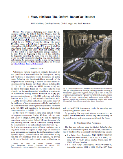 | W. Maddern, G. Pascoe, C. Linegar and P. Newman, "1 Year, 1000km: The Oxford RobotCar Dataset", The International Journal of Robotics Research (IJRR), 2016. [Bibtex][PDF] |
For documentation pertaining to the released ground truth, please refer to this follow-up paper:
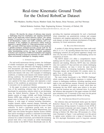 | W. Maddern, G. Pascoe, M. Gadd, D. Barnes, B. Yeomans, and P. Newman, "Real-time Kinematic Ground Truth for the Oxford RobotCar Dataset", in arXiv preprint arXiv: 2002.10152, 2020. [Bibtex][PDF] |
Dataset Description
Over the period of May 2014 to December 2015 we traversed a route through central Oxford twice a week on average using the Oxford RobotCar platform, an autonomous Nissan LEAF. This resulted in over 1000km of recorded driving with almost 20 million images collected from 6 cameras mounted to the vehicle, along with LIDAR, GPS and INS ground truth.
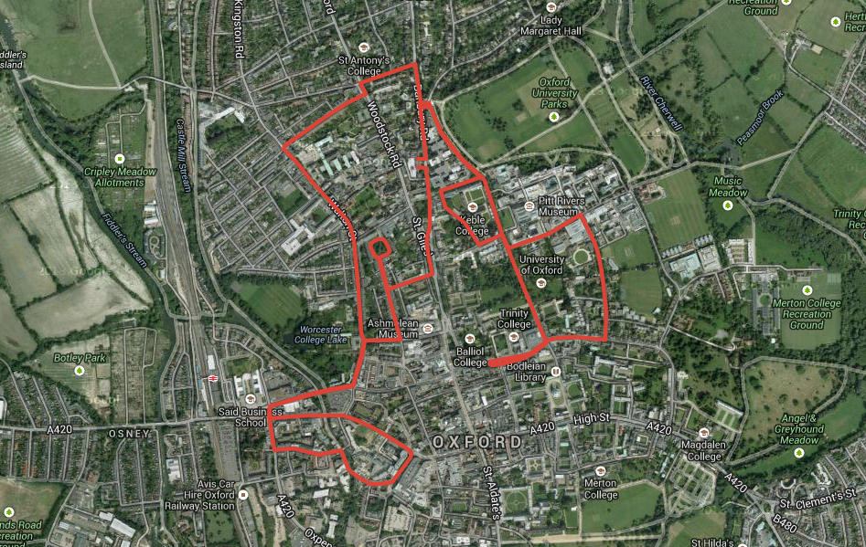
Map of the route used for dataset collection in central Oxford.
Data was collected in all weather conditions, including heavy rain, night, direct sunlight and snow. Road and building works over the period of a year significantly changed sections of the route from the beginning to the end of data collection.
By frequently traversing the same route over the period of a year we enable research investigating long-term localisation and mapping for autonomous vehicles in real-world, dynamic urban environments.
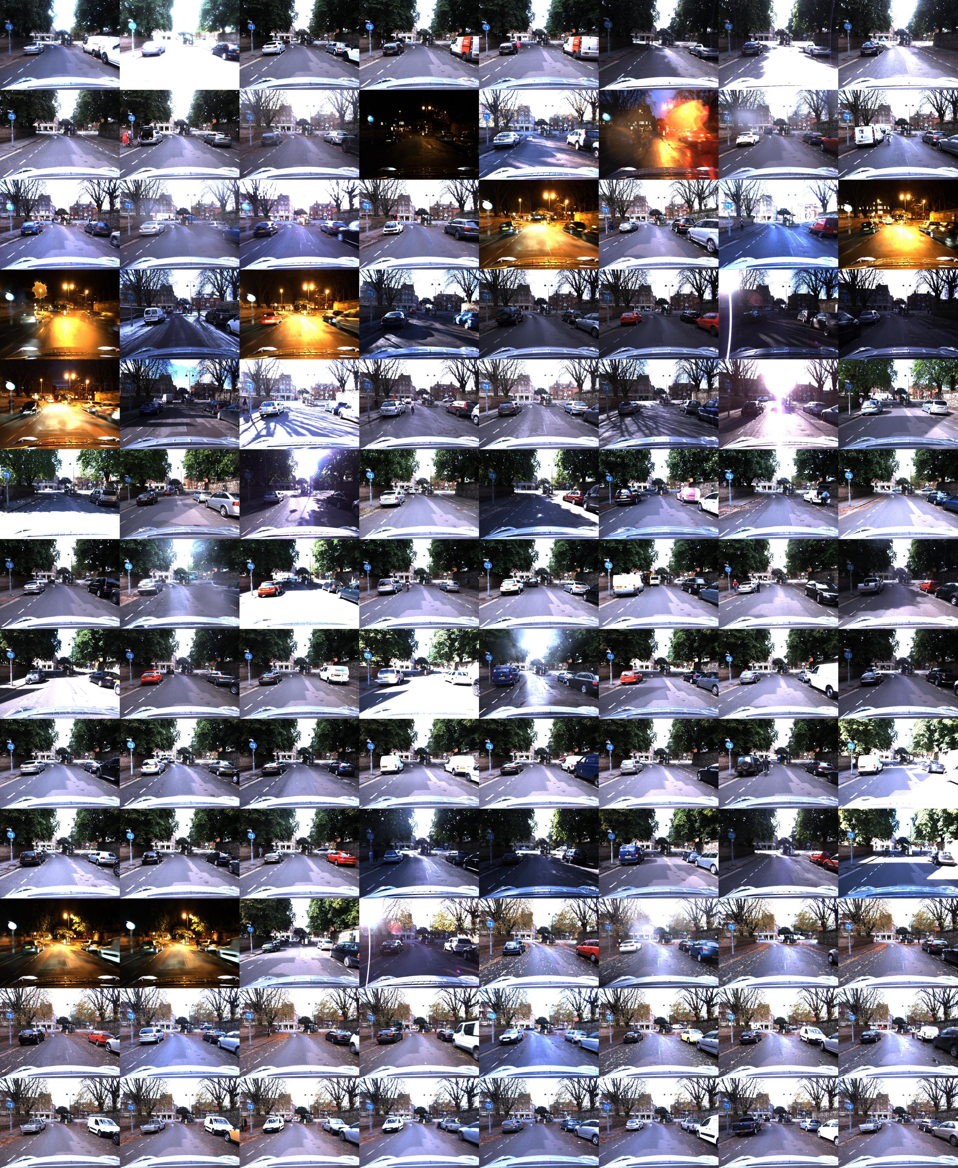
Sample images from different traversals in the dataset, showing variation in weather, illumination and traffic.
Sensor Suite
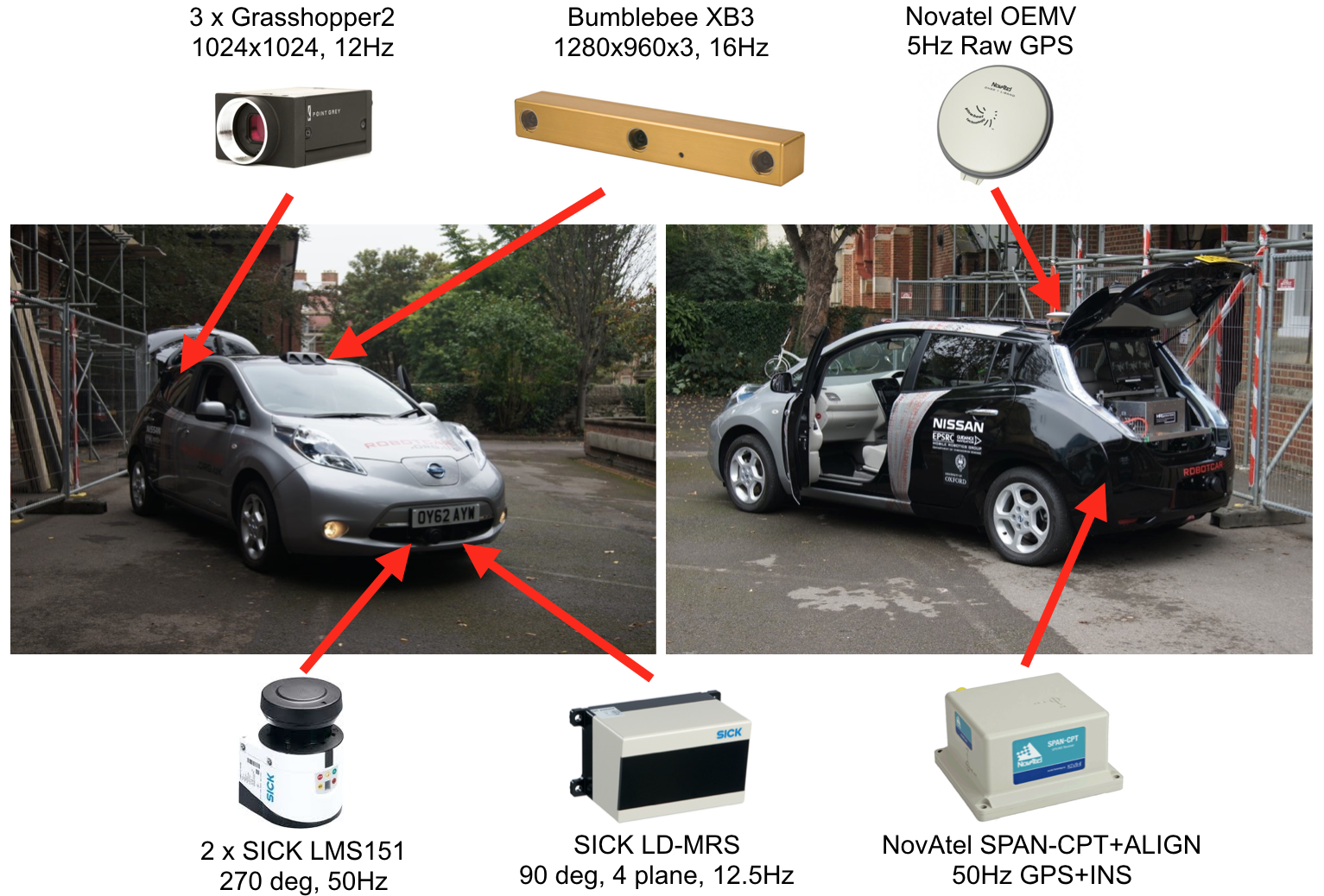
Sensors on the RobotCar
The RobotCar is equipped with the following sensors:
- Cameras:
- 1 x Point Grey Bumblebee XB3 (BBX3-13S2C-38) trinocular stereo camera, 1280×960×3, 16Hz, 1/3” Sony ICX445 CCD, global shutter, 3.8mm lens, 66° HFoV, 12/24cm baseline
- 3 x Point Grey Grasshopper2 (GS2-FW-14S5C-C) monocular camera, 1024×1024, 11.1Hz, 2/3” Sony ICX285 CCD, global shutter, 2.67mm fisheye lens (Sunex DSL315B-650-F2.3), 180° HFoV
- LIDAR:
- 2 x SICK LMS-151 2D LIDAR, 270° FoV, 50Hz, 50m range, 0.5° resolution
- 1 x SICK LD-MRS 3D LIDAR, 85° HFoV, 3.2° VFoV, 4 planes, 12.5Hz, 50m range, 0.125° resolution
- GPS/INS:
- 1 x NovAtel SPAN-CPT ALIGN inertial and GPS navigation system, 6 axis, 50Hz, GPS/GLONASS, dual antenna
Intrinsic calibration parameters and undistortion look-up-tables for the cameras are provided on the downloads page. For those wishing to perform their own calibrations, we also provide original images of a chequerboard sequence.
Sensor Locations
The below image shows the location and orientation of each sensor on the vehicle. Precise extrinsic calibrations for each sensor are included in the development tools.
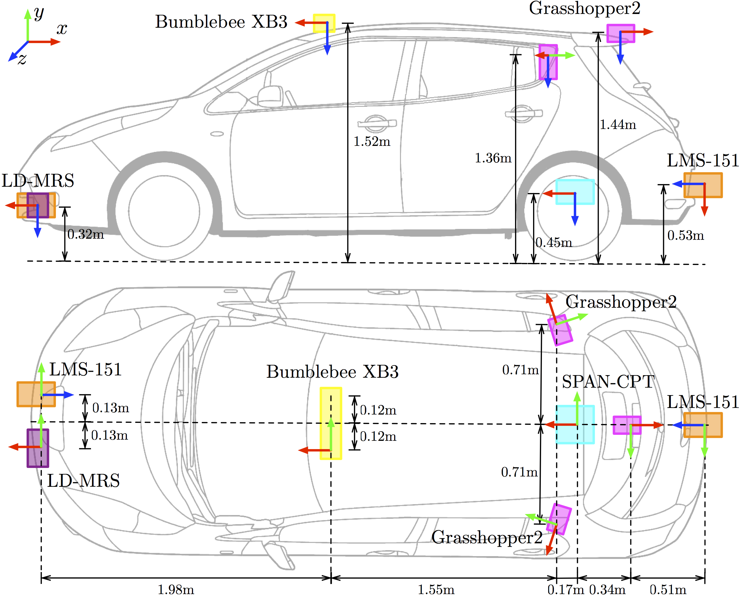
Sensor positions on vehicle. Coordinate frames use the convention x = forward (red), y = right (green), z = down (blue).
Data Format
For distribution we have divided up the datasets into individual routes, each corresponding to a single traversal. To reduce download file sizes, we have further divided up each traversal into chunks, where each chunk corresponds to an approximately 6 minute segment of the route. Within one traversal, chunks from different sensors will overlap in time (e.g. left stereo chunk 2 covers the same time period as LD-MRS chunk 2); however, chunks do not correspond between different traversals.

Directory structure of dataset downloads.
Each chunk has been packaged as a tar archive for downloading. It is intended that all tar archives are extracted in the same directory: this will preserve the folder structure indicated above when multiple chunks and/or traversals are downloaded. Each chunk archive also contains a full list of all sensor timestamps for the traversal in the <sensor>.timestamps file, as well as a list of condition tags as illustrated in the tags.csv file. The timestamps file contains ASCII formatted data, with each line corresponding to the UNIX timestamp and chunk ID of a single image or LIDAR scan.
Images
All images are stored as lossless-compressed PNG files in unrectified 8-bit raw Bayer format. The files are structured as <camera>/<sensor>/<timestamp>.png, where <camera> is stereo for Bumblebee XB3 images or mono for Grasshopper2 images, <sensor> is any of left | centre | right for Bumblebee XB3 images and left | rear | right for Grasshopper2 cameras, and <timestamp> is the UNIX timestamp of the capture, measured in microseconds.
The top left 4 pixel Bayer pattern for the Bumblebee XB3 images is GBRG, and for Grasshopper2 images is RGGB. The raw Bayer images can be converted to RGB using the MATLAB demosaic function, the OpenCV cvtColor function or similar methods.
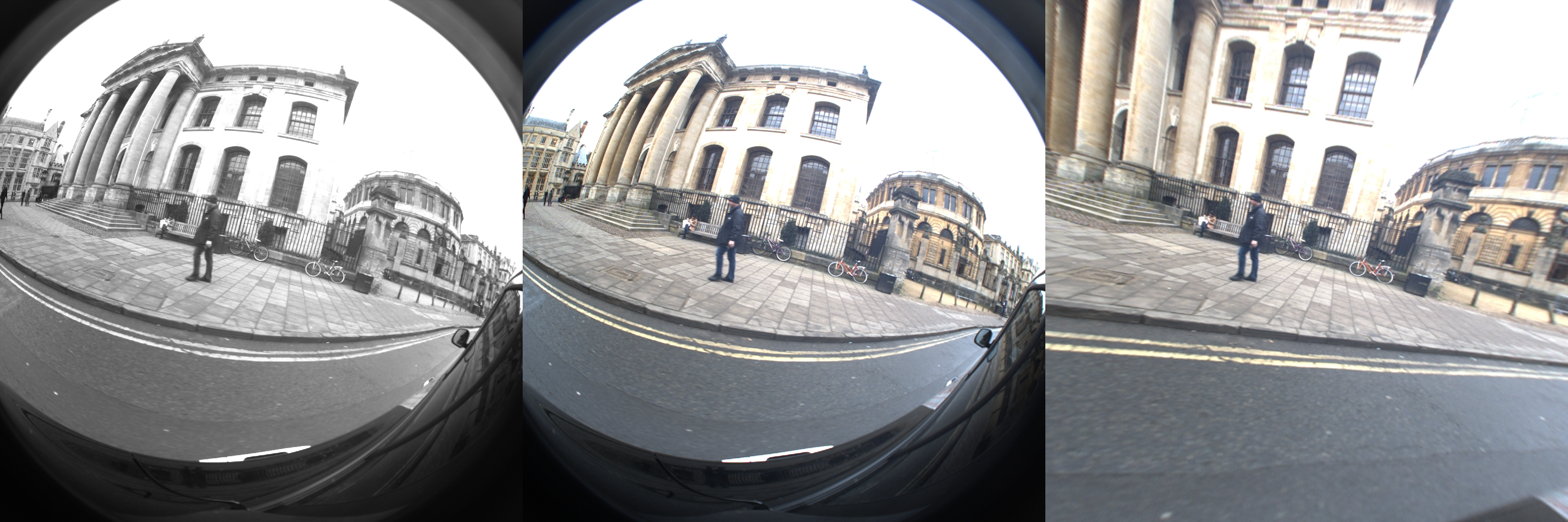
Image from one of the Grasshopper2 cameras. Left: image as provided; Centre: image after debayering; Right: center after undistortion.
LIDAR
2D LIDAR
The 2D LIDAR returns for each scan are stored as double-precision floating point values packed into a binary file, similar to the Velodyne scan format the KITTI dataset. The files are structured as <laser>/<timestamp>.bin, where <laser> is lms_front or lms_rear.
Each 2D scan consists of 541 triplets of (x, y, R), where x, y are the 2D Cartesian coordinates of the LIDAR return relative to the sensor (in metres), and R is the measured infrared reflectance value.
No correction for the motion of the vehicle has been performed when projecting the points into Cartesian coordinates; this can be optionally performed by interpolating a timestamp for each point based on the 15ms rotation period of the laser.
For a scan with filename <timestamp>.bin, the (x, y, R) triplet at index 0 was collected at <timestamp> and the triplet at index 540 was collected at <timestamp>+15e3.
3D LIDAR
The 3D LIDAR returns from the LD-MRS are stored in the same packed double-precision floating point binary format as the 2D LIDAR scans.
The files are structured as ldmrs/<timestamp>.bin. Each 3D scan consists of triplets of (x, y, z), which is the 3D Cartesian coordinates of the LIDAR return relative to the sensor (in metres). The LD-MRS does not provide infrared reflectance values for LIDAR returns.
GPS/INS
GPS and inertial sensor data from the SPAN-CPT are provided in an ASCII-formatted csv file. Two separate files are provided: gps.csv and ins.csv. gps.csv contains the GPS-only solution of latitude (deg), longitude (deg), altitude (m) and uncertainty (m) at 5Hz, and ins.csv contains the fused GPS+Inertial solution, consisting of 3D UTM position (m), velocity (m/s), attitude (rad) and solution status at 50Hz.
- Note
- The headers in
ins.csvgive the units of attitude as degrees. They are in fact in radians.
Visual Odometry (VO)
Local errors in the GPS+Inertial solution (due to loss or reacquisition of satellite signals) can lead to discontinuites in local maps built using this sensor as a pose source. For some applications a smooth local pose source that is not necessarily globally accurate is preferable.
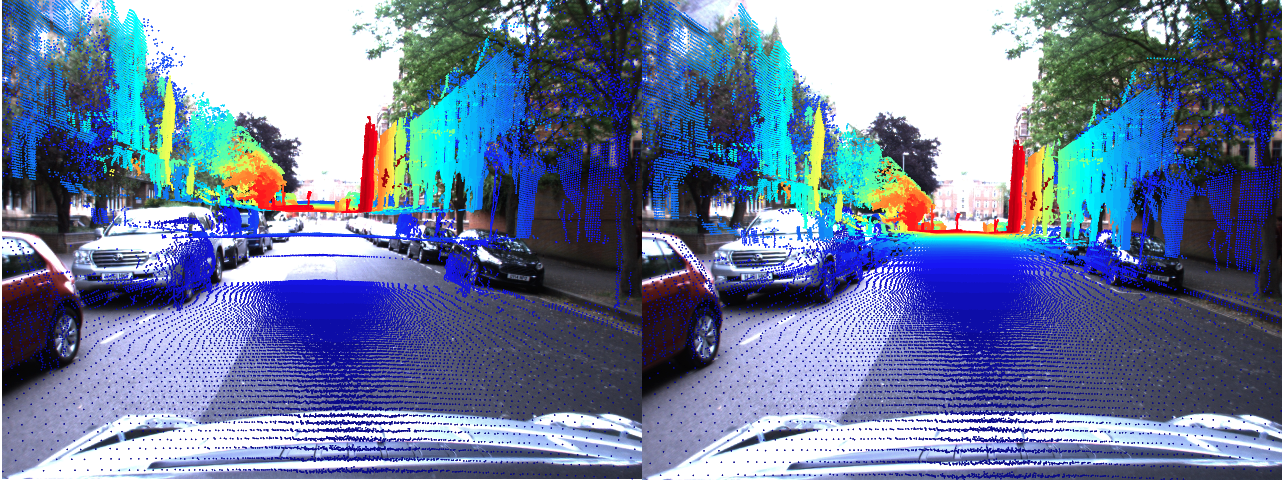
Projection of pointclouds into an image using pose estimate from the INS (left) and VO (right). The VO is not globally accurate, but provides a smooth, locally accurate relative pose estimate.
We have processed the full set of Bumblebee XB3 wide-baseline stereo imagery using our visual odometry system and provide the relative pose estimates as a reference local pose source. The file vo.csv contains the relative pose solution, consisting of the source and destination frame timestamps, along with the six-vector Euler parameterisation (x, y, z, α, β, γ) of the SE(3) relative pose relating the two frames. Our visual odometry solution is accurate over hundreds of metres (suitable for building local 3D pointclouds) but drifts over larger scales, and is also influenced by scene content and exposure levels; we provide it only as a reference and not as a ground truth relative pose system.
Development Kit
We provide a set of simple MATLAB and Python development tools for easy access to and manipulation of the dataset. The MATLAB and Python functions provided include simple functions to load and display imagery and LIDAR scans, as well as more advanced functions involving generating 3D pointclouds from push-broom 2D scans, and projecting 3D pointclouds into camera images.
Laser data projected into camera images using the software development kit.
Image Demosaicing and Undistortion
MATLAB
The function LoadImage.m reads a raw Bayer image from a specified directory and at a specified timestamp, and returns a MATLAB format RGB colour image. The function can also take an optional look-up table argument (provided by the function ReadCameraModel.m) which will then rectify the image using the undistortion look-up tables.
Python
The load_image function in the image module will load and image, perform Bayer demosaicing, and optionally undistort the image. A camera model for undistortion can be built with the CameraModel class.
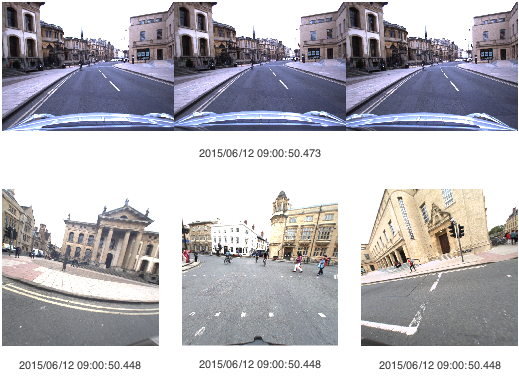
Image playback using the development kit.
3D Pointcloud Generation
The function BuildPointcloud.m (MATLAB) or build_pointcloud (Python) combines a 6DoF trajectory from the INS with 2D LIDAR scans to produce a local 3D pointcloud. The resulting pointcloud is coloured using LIDAR reflectance information, highlighting lane markings and other reflective objects. The size of the pointcloud can be controlled using the start_timestamp and end_timestamp arguments.
In MATLAB, BuildPointcloud can be called without outputs to visualise the pointcloud. The Python build_pointcloud.py script can be run from the command line to display the 3D pointcloud.
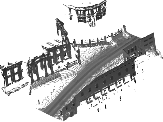
Pointcloud generated using the development kit.
Pointcloud Projection Into Images
MATLAB
The function ProjectLaserIntoCamera.m combines the above two tools as follows: LoadImage.m is used to retrieve and undistort a raw image from a specified directory at a specified timestamp, then BuildPointcloud.m is used to generate a local 3D pointcloud around the vehicle at the time of image capture. The 3D pointcloud is then projected into the 2D camera image using the camera intrinsics.
Python
The same functionality is provided by the project_laser_into_camera.py script. The CameraModel class provides both image undistortion and pointcloud projection, using a pinhole camera model.

Pointcloud projected into a camera image.